Understanding LLM Inference Performance: Latency, Throughput, and Goodput

When discussing LLM serving performance, “fast” has at least three meanings: how long users wait to see the first token and whether subsequent tokens arrive smoothly; how much work the system can complete per unit time; and how many requests actually meet their latency targets. This article starts from the prefill and decode stages of a single request and introduces TTFT, TPOT, ITL, E2E latency, throughput, SLOs, and goodput in turn, explaining why peak throughput does not necessarily mean a good online service.

This article discusses only latency, throughput, and service levels in LLM serving. It does not cover answer quality, safety, or inference cost.

1. Starting from a single LLM request: Prefill and Decode

After a user sends an LLM request, the model does not directly “write” the entire answer continuously. It roughly goes through two stages: first understanding the input, then generating the output step by step.

1.1 Prefill: processing the input

During prefill, the model processes the user’s prompt and computes and stores intermediate results for its tokens. These results are stored in the KV cache for later generation.

The longer the prompt, the more input the model must process, so this preparation stage usually takes longer. It can be understood as the model “reading the question and building the context.”

1.2 Decode: generating step by step

After processing the input, the model enters the decode stage. It generates one new token from the context so far, adds that token to the context, and continues with the next token:

y_1 \rightarrow y_2 \rightarrow y_3 \rightarrow \cdots

Because each token depends on the preceding content, decode usually cannot be parallelized as broadly as input processing. The KV cache prevents the model from recomputing the context it has already processed, but the model still needs to repeatedly read the cache and generate new tokens.

This stage can be understood as the model “writing the answer one word at a time.” The longer the output, the longer decode usually continues.

An individual request can therefore be represented simply as:

\text{Request arrives} \rightarrow \text{Prefill: process input} \rightarrow \text{Decode: generate output} \rightarrow \text{Request completes}

Prefill and decode have different computational characteristics: the former resembles processing a large amount of input at once, while the latter repeatedly performs small steps. This difference is why LLM serving must consider both the user’s waiting time and the system’s overall throughput. The following sections introduce the metrics used to measure these aspects.

2. Latency and Throughput

Once prefill and decode are clear, we can ask whether an LLM inference system is “fast.” There are two distinct perspectives:

From the user’s perspective, we care about how long one request takes. This is latency.
From the system’s perspective, we care about how much work can be completed per unit time. This is throughput.

Latency and throughput are not the same problem. A system can give a small number of users very low latency, or use batching to serve many users at once and achieve high aggregate throughput, but it is difficult to maximize both under every load level.

2.1 Latency: how long does one request take?

Latency describes the response time of an individual request and directly affects the user experience of interactive applications such as chat and code completion. For streaming generation, common latency metrics include:

TTFT (Time to First Token): the time from the measurement starting point until the first output token is received. It is affected mainly by request queueing, scheduling, prefill computation, and first-token sampling. A lower TTFT means the user sees the response begin sooner.
ITL (Inter-Token Latency): the interval between two adjacent output tokens. ITL describes the duration of each pause during streaming generation. Lower and less variable ITL generally produces smoother output.
TPOT (Time per Output Token): after the first token is returned, the average time needed to generate each subsequent token. It can be understood as the average ITL of one request during decode.
E2E Latency (End-to-End Latency): the total time from the measurement starting point until the complete response finishes.

The “measurement starting point” must be stated explicitly in a benchmark. A client-side measurement usually begins when the request is sent and includes network and protocol overhead. A server-side measurement may begin when the service receives the request and focus more narrowly on the serving system itself. Latency numbers are directly comparable only when their measurement boundaries are consistent.

The following figure shows the measurement range of each latency metric in a streaming generation request:

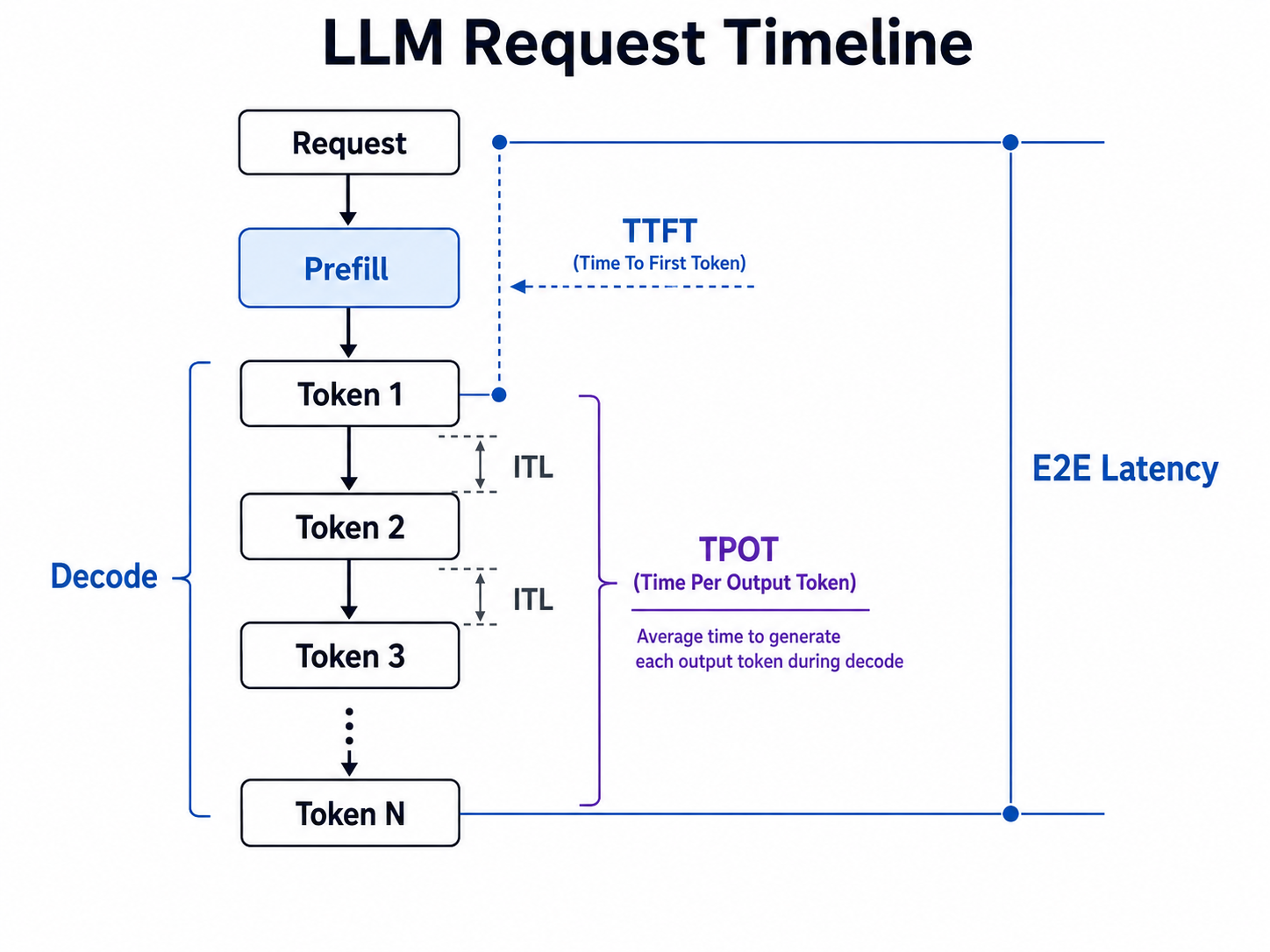
Timeline of TTFT, ITL, TPOT, and E2E latency in an LLM request

Figure: TTFT describes when an answer begins, ITL and TPOT describe the generation speed while it is produced, and E2E latency describes the total time required by the request.

If a request generates $N$ output tokens, then—ignoring small measurement errors—we can approximate:

\text{E2E Latency} \approx \text{TTFT} + (N-1)\times\text{TPOT}

This relationship shows that TTFT accounts for a larger share of the experience for short answers, while TPOT during continuous generation gradually becomes the main contributor to E2E latency for long answers.

2.2 Throughput: how much work can the whole system process?

If latency asks how fast one request is, throughput asks how much work the inference system can complete per unit time. It represents the service capacity of the system as a whole.

Request Throughput

Request throughput measures the number of requests completed by the system per unit time. It is usually expressed in $requests/s$ , also known as RPS (requests per second):

\text{Request Throughput} = \frac{\text{Completed Requests}}{\text{Measurement Duration}}

RPS can reflect a system’s ability to handle concurrent requests, but it does not capture the amount of work contained in each request. Generating a short greeting and generating a long article clearly impose different computational loads. Comparing RPS directly can therefore be misleading when input lengths, output lengths, or traffic patterns differ.

Factors that affect RPS include:

Prompt length and generation length
Model size, numerical precision, and hardware configuration
Batch size, concurrency, and request-arrival pattern
Optimizations such as prefix caching and speculative decoding
Scheduling and memory-management capabilities of the inference engine

Token Throughput

Token throughput measures the number of tokens processed or generated by the system per unit time. It is usually expressed in $tokens/s$ , also known as TPS (tokens per second). Depending on what is counted, it can be divided further into:

Input Token Throughput: the number of input tokens actually processed by the system per unit time.
Output Token Throughput: the number of output tokens generated by the system per unit time.
Total Token Throughput: the combined throughput of input and output tokens.

LLM performance discussions must also distinguish single-user generation speed from aggregate system throughput:

Per-user Output Token Rate describes how many output tokens an individual request receives per second. During steady-state generation, it is approximately $1/\text{TPOT}$ .
Aggregate Output Token Throughput describes the total number of output tokens generated per second across all concurrent requests.

Increasing concurrency may raise aggregate TPS while making TPOT worse for each user. “How many tokens the system generates per second” and “how quickly one user sees text appear” are therefore two different questions.

Input TPS and output TPS also matter differently for different workloads:

For long-input, relatively short-output tasks such as long-document summarization, prefill represents a larger share of the work, so input TPS deserves more attention.
For short-prompt, long-output tasks such as chat or content generation, decode represents a larger share, making output TPS and per-user TPOT more important.

Changing input and output lengths changes the balance of prefill and decode work, so TPS measured under different length distributions cannot be compared directly. At minimum, a benchmark should clarify whether TPS means input, output, or total TPS, and whether it represents single-request speed or aggregate system throughput.

As batch size and the number of concurrent requests increase, aggregate system TPS usually rises at first, until compute capacity, memory capacity, or memory bandwidth becomes saturated. Beyond the saturation point, adding more requests may not improve realized throughput. Instead, queues may grow, latency may deteriorate, and requests may time out or fail.

3. From Throughput to Goodput: what counts as “good” under high concurrency?

Real LLM serving systems usually trade throughput against latency. Larger batches and higher concurrency can improve GPU utilization and aggregate system throughput, but they can also increase queueing time and resource contention, worsening TTFT, TPOT, or tail latency.

Evaluating an online service therefore requires more than asking about peak throughput. We must also ask: how many requests can the system sustain while meeting the product’s latency requirements? To answer this question, we need latency distributions, SLOs, and goodput.

3.1 Why can higher Throughput make users slower?

When a single request is decoding, each step generates only one new token and performs relatively little work, which usually cannot fully utilize a GPU. Serving systems therefore place multiple requests in the same batch so that one model execution serves several sequences at once.

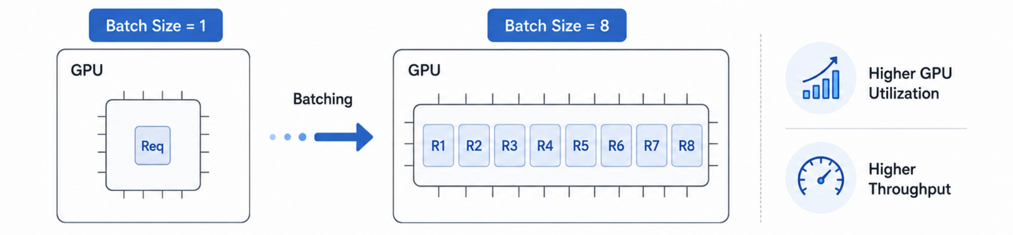
Increasing batch size from 1 to 8 improves GPU utilization and system throughput

Figure: batching lets multiple requests share one model execution, helping improve GPU utilization and aggregate throughput.

Batching is not free, however. As system load increases, new requests may wait in a queue, while new prefill work may compete with active decode work for execution time and hardware resources. Higher concurrency and larger batches can therefore produce all of the following at once:

Higher request throughput and aggregate TPS
Longer queueing time and TTFT
Worse TPOT or more variable token intervals
More severe tail latency

Sarathi-Serve studies this throughput–latency trade-off directly. Decode batching benefits system throughput, but interleaving prefill and decode within the same serving engine can also create latency interference. The paper mitigates this problem with chunked prefill and stall-free batching. (arXiv)

The following simplified curve illustrates how latency changes as load increases:

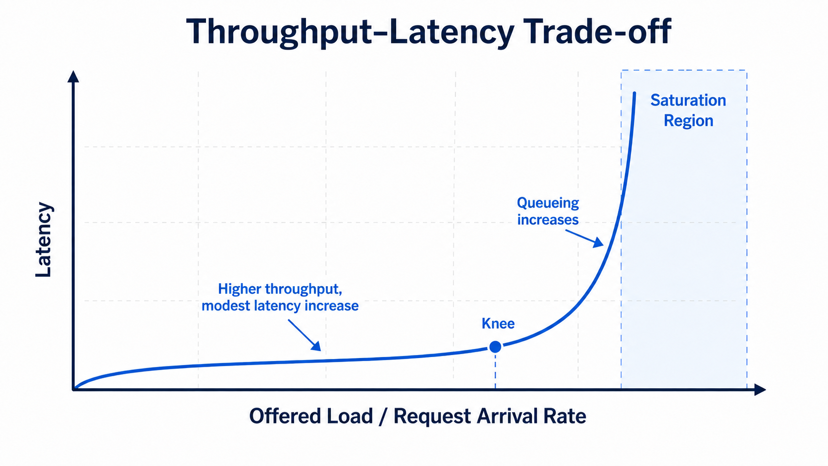
Latency rises rapidly near saturation as request load increases

Figure: at low load, raising the request arrival rate increases throughput with little change in latency. Near saturation, queues grow rapidly and latency deteriorates sharply.

This shows why running a GPU at full utilization does not necessarily imply a good user experience. Under high concurrency, system throughput and per-request latency must be considered together.

3.2 A single average hides tail latency

Even after we begin examining latency, an average alone is not enough. Mean latency tells us how long all requests wait on average, but it does not show how those delays are distributed among requests. Two systems with the same mean latency can deliver completely different experiences.

Suppose two systems each process 100 requests:

System	Request latency distribution	Mean latency
A	All 100 requests take 200 ms	200 ms
B	98 requests take 100 ms; 2 take 5.1 s	200 ms

Every request in System A finishes in 200 ms. Most requests in System B are faster, but 2% take 5.1 seconds. The mean is identical, so mean alone cannot distinguish these very different distributions.

Online services therefore also examine latency percentiles such as the median, P90, P95, and P99. The following is a common right-skewed latency distribution: most requests cluster in the low-latency region on the left, while a few requests spread out to the right and form a long tail.

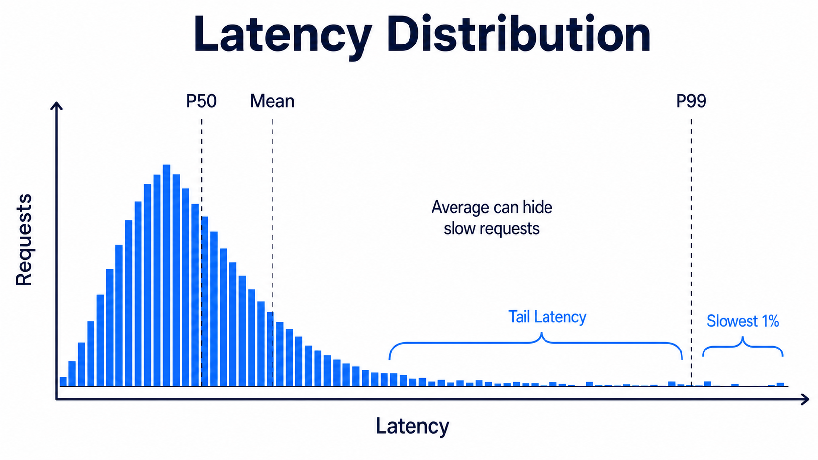
P50, P99, and tail latency in a right-skewed latency distribution

Figure: P50 describes the center of the latency distribution, the mean is pulled upward by slow requests on the right, and high percentiles such as P95 and P99 expose the tail.

These statistics answer different questions:

Mean: the sum of all observations divided by the number of requests. It describes the overall average but is sensitive to extreme values.
Median / P50: half of the requests have latency at or below this value. It commonly describes where a typical request lies.
P95 / P99: at least approximately 95% / 99% of requests have latency at or below these values. They are commonly used to quantify the high-latency tail.

Using TTFT as an example:

P99(\mathrm{TTFT}) = 2\text{s}

means that, for the current sample and percentile method, approximately 99% of requests have a TTFT no greater than two seconds. The remaining 1% may be slower—potentially much slower.

The high-latency requests on the right side of the distribution are generally described as tail latency. Production systems care about the tail because a small number of severely delayed requests can still damage service reliability, even when the vast majority are fast. High percentiles such as P95 and P99 are common ways to quantify it.

Percentiles still only describe how slow the system became; they do not automatically tell us whether that latency is acceptable for the product. To decide whether a service is fast enough, we need explicit targets for these metrics—this leads to SLOs.

3.3 SLO: how fast is “good enough”?

The same two-second TTFT may be perfectly acceptable for offline document summarization but noticeably disruptive for real-time code completion in an IDE. A production system therefore cannot express its objective simply as:

\text{Latency} \rightarrow \text{as low as possible}

Instead, it must set measurable and verifiable targets for key metrics based on the product scenario. This is a Service Level Objective (SLO).

It is useful to distinguish two related concepts:

A Service Level Indicator (SLI) is an actually measured service metric, such as a P99 TTFT of 1.7 seconds.
An SLO is the target that an SLI should meet, such as a P99 TTFT no greater than two seconds.

For example, an interactive application might require:

P99(\mathrm{TTFT}) \le 2\text{s} \qquad P99(\mathrm{TPOT}) \le 50\text{ms}

This is an aggregate percentile objective: under a specified measurement window and workload, it requires approximately 99% of requests to stay within the corresponding latency boundaries. An SLO turns the abstract goal of “responsive and smooth generation” into a service target that can be verified.

Standardized benchmarks use similar designs. For example, MLPerf Inference v6.0 sets latency constraints of P99 TTFT ≤ 2.0 s and TPOT ≤ 15 ms for the GPT-OSS 120B Interactive scenario, and P99 TTFT ≤ 1.5 s and TPOT ≤ 15 ms for DeepSeek-R1 Interactive. These thresholds apply only to their corresponding models, datasets, and scenarios and should not be copied directly into every LLM application, but they demonstrate the role of an SLO well. (MLCommons)

In addition to aggregate percentile objectives, goodput benchmarks often use per-request qualification thresholds. For example, a request may be required to satisfy both:

\mathrm{TTFT} \le 2\text{s} \qquad \mathrm{TPOT} \le 50\text{ms}

Only a request satisfying both conditions is considered qualifying.

With an SLO, the question changes from “which system has lower latency?” to how many qualifying requests can the system complete per second while meeting the product’s latency requirements? That is the question goodput answers.

3.4 Goodput: effective throughput that meets SLOs

Throughput counts how many requests the system completes per second. Goodput counts only the requests that meet every per-request SLO. AIPerf defines it as:

\text{Goodput} = \frac{\text{Requests Meeting All SLOs}} {\text{Benchmark Duration}}

If a request meets the TTFT target but exceeds the TPOT threshold, it is still excluded from goodput. Therefore:

0 \le \text{Goodput} \le \text{Request Throughput}

In other words, throughput measures how quickly the system completes work, while goodput measures how quickly it completes work that meets the predefined service targets. (NVIDIA Docs)

Suppose we test two serving systems under the same workload, duration, and SLOs:

System	Request Throughput	Goodput	SLO pass rate
Server A	100 req/s	60 req/s	60%
Server B	85 req/s	80 req/s	94.1%

Server A has higher raw throughput, but under heavy load many of its requests violate the latency SLOs, leaving only 60 qualifying requests per second. Server B has slightly lower raw throughput, yet 80 requests per second meet every SLO. If the goal is stable service under the specified latency constraints, Server B has greater effective service capacity.

DistServe goes further and treats this idea as an optimization objective for LLM serving. Given an application’s TTFT and TPOT requirements, the system should optimize the maximum request rate it can sustain under those latency constraints, rather than only pursuing unconstrained peak throughput. DistServe separates prefill and decode to reduce interference between the two stages and optimize their resource configurations independently. (arXiv)

The vLLM Benchmark CLI also provides a --goodput option for setting per-request thresholds for ttft, tpot, and e2el in milliseconds. For example, adding the following to a complete vllm bench serve command:

--goodput ttft:2000 tpot:50

means that only requests with TTFT no greater than 2,000 ms and TPOT no greater than 50 ms count toward goodput. If either condition is violated, the request does not qualify. Other benchmark parameters—such as the model, backend, dataset, and request rate—are omitted here. (vLLM)

3.5 How does Goodput change with system load?

Goodput is not a fixed number independent of test conditions. It changes with request arrival rate, concurrency, input and output lengths, and SLO thresholds.

At low load: requests spend almost no time queueing and most meet their SLOs, so goodput is usually close to request throughput.
Near saturation: request throughput may still rise, but queueing and resource contention begin to increase TTFT, TPOT, and tail latency. The two curves gradually diverge.
After overload: request throughput often approaches a plateau, while goodput may stop growing or even decline because more requests finish only after violating an SLO.

The following figure shows a typical relationship between throughput and goodput as offered load increases:

Throughput and goodput curves as offered load increases

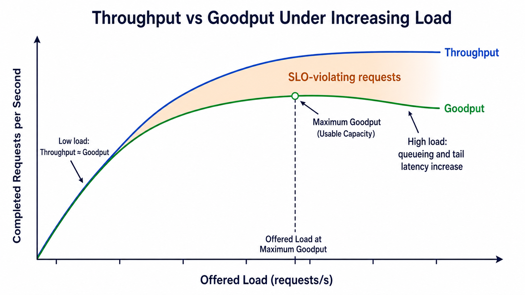
Figure: throughput and goodput are close at low load. As load increases, more requests violate SLOs and the two curves diverge.

The peak of the green curve is the maximum goodput measured under the current test conditions. The offered load at that peak can be understood as the load level near the boundary of the system’s usable capacity.

This also shows why a goodput report must include its test conditions, at least:

Model, precision, inference engine, and hardware configuration
Input and output length distributions
Request-arrival pattern, request rate, and maximum concurrency
TTFT, TPOT, E2E, or other SLO thresholds
Benchmark duration, warm-up procedure, and request count
Handling of timed-out, failed, and cancelled requests

Two goodput numbers are comparable only when these conditions are substantially aligned. Ultimately, we do not care how much work can be “stuffed into” the system without regard for latency. We care about:

\boxed{ \text{How much effective throughput can the system sustain while meeting its latency SLOs?} }

4. Summary

Evaluating an LLM serving system requires moving from the experience of one request to the behavior of the whole system:

TTFT, TPOT, ITL, and E2E latency describe how long each stage of one request takes.
Mean, P50, P95, and P99 describe the latency distribution across many requests, separating average experience, typical experience, and tail latency.
Request throughput and token throughput describe how many requests the system completes or how many tokens it processes per unit time.
An SLO sets the boundary that the product considers acceptable for these metrics.
Goodput describes how many requests per unit time actually satisfy all per-request SLOs.

The relationship among these concepts can be summarized as:

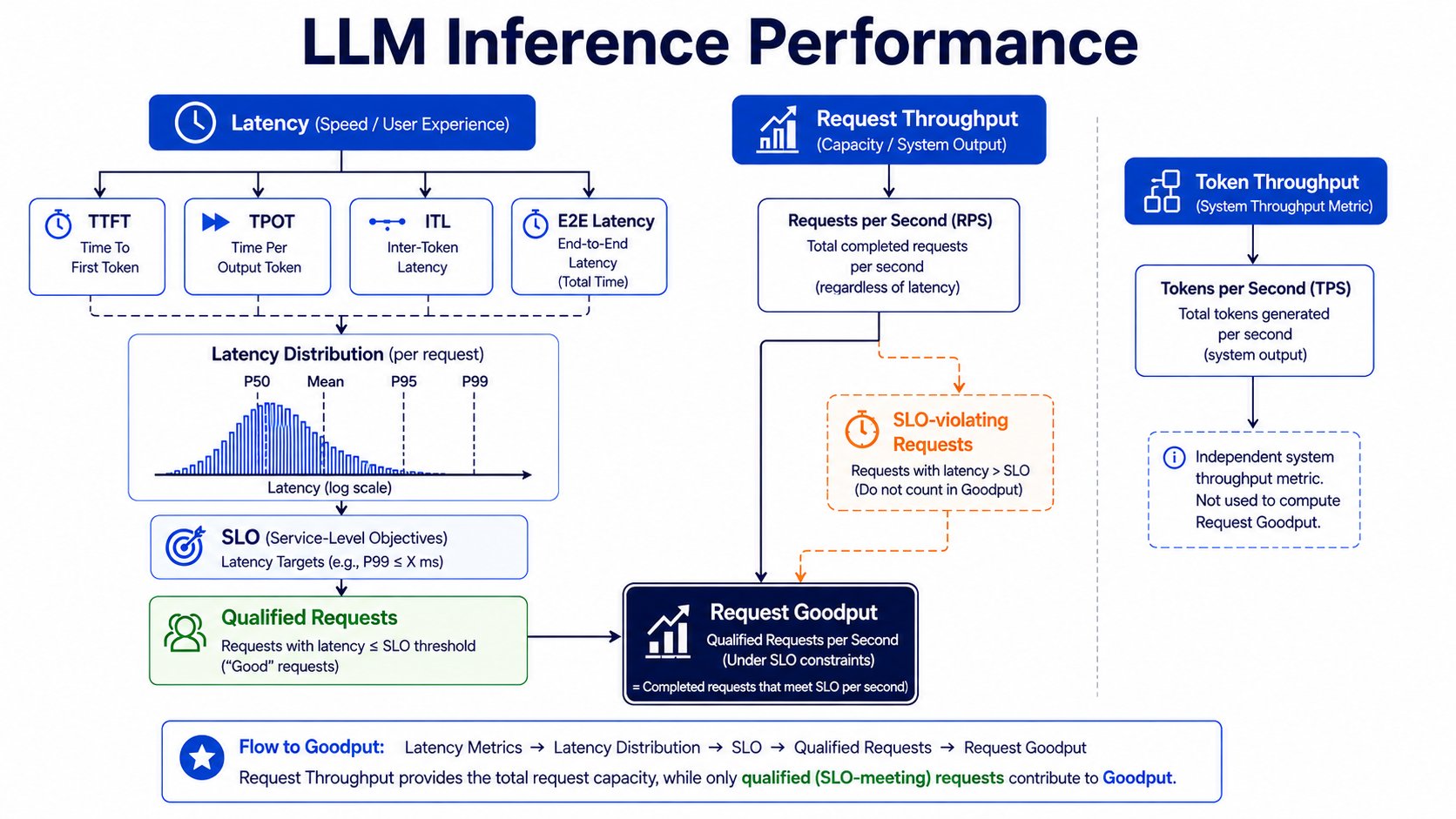
\text{Latency Metrics} \rightarrow \text{Latency Distribution} \xrightarrow{\text{SLO}} \text{Qualifying Requests} \xrightarrow{\text{Count per Unit Time}} \text{Goodput}

The relationship between latency, throughput, SLOs, and goodput in LLM inference

Figure: latency describes the experience of one request, throughput describes system capacity, an SLO defines the qualification boundary, and goodput measures effective request throughput within that boundary.

References

Key metrics for LLM inference (LLM Inference Handbook)
vLLM — Metrics (vLLM)
vLLM — vllm bench serve (vLLM)
NVIDIA AIPerf Metrics Reference (NVIDIA Docs)
MLPerf Inference v6.0 — GPT-OSS and DeepSeek-R1 Interactive scenarios (MLCommons)
DistServe: Disaggregating Prefill and Decoding for Goodput-optimized Large Language Model Serving (arXiv)
Taming Throughput-Latency Tradeoff in LLM Inference with Sarathi-Serve (arXiv)